Speed-Time Graphs
This is a lesson summary. The full lesson can be viewed by purchasing an online course subscription.
Learning Objective
In this lesson we will learn how changes in speed can be represented graphically.
Learning Outcomes
By the end of this lesson you will be able to:
- Describe the layout of a speed-time graph.
- Describe how constant speed, increasing speed, decreasing speed and stationariness are represented on a speed-time graph.
- Describe the relationship between the gradient of the line on a speed-time graph and acceleration.
- Calculate acceleration from a speed-time graph.
- Calculate distance travelled from a speed-time graph.

(Image: PublicDomainPictures, Pixabay)
Lesson Summary
- A speed-time graph plots the speed of an object (on the y-axis) against time (on the x-axis).
- Speed-time graphs can show:
- Stationariness – a horizontal line that lies on the x-axis (y = 0).
- Constant speed – a horizontal line that lies above the x-axis (y > 0).
- Increasing speed (acceleration) – a line with a positive gradient.
- For constant acceleration, the line will be straight.
- Decreasing speed (deceleration) – a line with a negative gradient.
- For constant deceleration, the line will be straight.
- The gradient of the line on a speed-time graph represents acceleration.
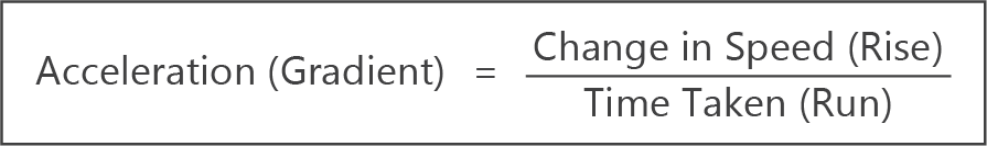
- The steeper the slope of the line on a speed-time graph, the greater the acceleration.
- The area under the line on a speed-time graph represents distance travelled.
- For rectangular sections, distance (area) = speed × time.
- For triangular sections, distance (area) = ½ × speed × time.
- For speed-time graphs containing multiple rectangular and triangular sections, the total distance travelled is given by the combined areas of these sections.

(Image: Realbigtaco, Wikimedia Commons)
(Header image: Andrr, Adobe Stock)